When you start to use Armadillo as a backend for DataSHIELD you can
use the DSMolgenisArmadillo package for research purposes.
There is a default workflow in DataSHIELD to do analysis. These are the
steps that you need to take:
Authenticate
First obtain a authentication credentials from the authentication server to authenticate in DataSHIELD. These credentials contain an access token along with an authentication token which is used to refresh the session if it has timed out.
# Load the necessary packages.
library(dsBaseClient)
library(DSMolgenisArmadillo)

# specify server url
armadillo_url <- "https://armadillo-demo.molgenis.net"

# get token from central authentication server
token <- armadillo.get_credentials(armadillo_url)
#> [1] "We're opening a browser so you can log in with code V6TRZV"
Then build a login dataframe and perform the login on the Armadillo
server. The important part is to specify the driver. This should be
ArmadilloDriver.
# build the login dataframe
builder <- DSI::newDSLoginBuilder()
builder$append(
  server = "armadillo",
  url = armadillo_url,
  token = token@access_token,
  driver = "ArmadilloDriver",
  profile = "xenon",
  )

# create loginframe
login_data <- builder$build()

# login to server
conns <- DSI::datashield.login(logins = login_data, assign = FALSE)
Authenticate (legacy)
In previous versions of DSMolgenisArmadillo token
refreshing was not possible and tokens were requested using
armadillo.get_token.
# Load the necessary packages.
library(dsBaseClient)
library(DSMolgenisArmadillo)

# specify server url
armadillo_url <- "https://armadillo-demo.molgenis.net"

# get token from central authentication server
token <- armadillo.get_token(armadillo_url)
#> [1] "We're opening a browser so you can log in with code NFRDG5"
# Build login dataframe
builder <- DSI::newDSLoginBuilder()

builder$append(
  server = "armadillo",
  url = armadillo_url,
  token = token,
  driver = "ArmadilloDriver",
  profile = "xenon",
  )

login_data <- builder$build()

# login to server
conns <- DSI::datashield.login(logins = login_data, assign = FALSE)
You can append multiple servers to the login frame to perform an analysis across multiple cohorts.
Assign data
To work with DataSHIELD you need to be able to query data. You can do this by assigning data in the Armadillo service.
Assign data using expressions
You can assign values from expressions to symbols.
# assign some data to 'K'
datashield.assign.expr(conns = conns, symbol = "K", "c(10,50,100)")
# calculate the mean of 'K' to see that the assignment has worked
ds.mean("K", datasources = conns)
#> $Mean.by.Study
#>           EstimatedMean Nmissing Nvalid Ntotal
#> armadillo      53.33333        0      3      3
#>
#> $Nstudies
#> [1] 1
#>
#> $ValidityMessage
#>           ValidityMessage
#> armadillo "VALID ANALYSIS"
Assign data from tables
You can check which tables (data.frame’s) are available
on the Armadillo.
datashield.tables(conns)
#> $armadillo
#>   [1] "examplelink5/test-sub/non_rep"               "examplelink5/test-sub/yearly_rep"
#>   [3] "my-link/eos-demo/table"                      "examplelink11/test-sub/non_rep"
#>   [5] "examplelink11/test-sub/yearly_rep"           "examplelink13/test-sub/non_rep"
#>   [7] "examplelink13/test-sub/yearly_rep"           "examplelink14/test-sub/non_rep"
#>   [9] "examplelink14/test-sub/yearly_rep"           "examplelink9/test-sub/non_rep"
#>  [11] "examplelink9/test-sub/yearly_rep"            "nch3o1r0zn/2_1-core-1_0/trimesterrep"
#>  [13] "nch3o1r0zn/2_1-core-1_0/nonrep"              "nch3o1r0zn/2_1-core-1_0/yearlyrep"
#>  [15] "nch3o1r0zn/2_1-core-1_0/monthlyrep"          "nch3o1r0zn/1_1-outcome-1_0/nonrep"
#>  [17] "nch3o1r0zn/1_1-outcome-1_0/yearlyrep"        "nch3o1r0zn/survival/veteran"
#>  [19] "chop/2_6_core_1_3/non_rep"                   "chop/2_6_core_1_2/non_rep"
#>  [21] "chop/2_6_core_1_1/non_rep"                   "examplelink8/test-sub/non_rep"
#>  [23] "examplelink8/test-sub/yearly_rep"            "new-subset-folder/data/mtcars-2"
#>  [25] "genr/2_5-core-6_0/non_rep"                   "genr/2_5_core_6_0/non_rep"
#>  [27] "testsubset/core/testtable"                   "testsubset/core/yearlyrep"
#>  [29] "testsubset/core/nonrep"                      "test-ds-upload/test_data/mtcars"
#>  [31] "study1/core/year_rep"                        "study1/core/non_rep"
#>  [33] "study1/outcome/year_rep"                     "lifecycle/core/nonrep"
#>  [35] "lifecycle/core/yearlyrep"                    "gecko/2_1-core-1_0/trimesterrep"
#>  [37] "gecko/2_1-core-1_0/nonrep"                   "gecko/2_1-core-1_0/yearlyrep"
#>  [39] "gecko/2_1-core-1_0/monthlyrep"               "gecko/1_3_outcome_ath_1_0/trimester_rep"
#>  [41] "gecko/1_3_outcome_ath_1_0/non_rep"           "gecko/1_1-outcome-1_0/nonrep"
#>  [43] "gecko/1_1-outcome-1_0/yearlyrep"             "gecko/test-lt/LT_example_data"
#>  [45] "link-test/core-variables/nonrep"             "ds-workshop-24/data/selfesteem"
#>  [47] "ds-workshop-24/data/CNSIM2"                  "ds-workshop-24/data/CNSIM3"
#>  [49] "ds-workshop-24/data/test_link"               "ds-workshop-24/data/CNSIM1"
#>  [51] "examplelink10/test-sub/non_rep"              "examplelink10/test-sub/yearly_rep"
#>  [53] "study2/core/year_rep"                        "fix-subset/core/testtable"
#>  [55] "examplelink12/test-sub/non_rep"              "examplelink12/test-sub/yearly_rep"
#>  [57] "examplelink6/test-sub/non_rep"               "examplelink6/test-sub/yearly_rep"
#>  [59] "test/data/mtcars"                            "test/data/LT-example-dataset_long-format"
#>  [61] "test/data/d"                                 "test/view/view-tabel"
#>  [63] "test/test/test"                              "armadillo-illustration/barcelona/pancreatic"
#>  [65] "armadillo-illustration/groningen/pancreatic" "trajectories/data/alspac"
#>  [67] "trajectories/data/chs"                       "trajectories/data/bib"
#>  [69] "trajectories/data/bcg"                       "trajectories/data/probit"
#>  [71] "ninfea/2_7_core_1_2/yearly_rep"              "ninfea/2_7_core_1_2/monthly_rep"
#>  [73] "ninfea/2_7_core_1_2/trimester_rep"           "ninfea/2_7_core_1_2/non_rep"
#>  [75] "ninfea/2_7_core_1_4/non_rep"                 "ninfea/2_7_core_1_1/yearly_rep"
#>  [77] "ninfea/2_7_core_1_1/monthly_rep"             "ninfea/2_7_core_1_1/trimester_rep"
#>  [79] "ninfea/2_7_core_1_1/non_rep"                 "ninfea/1_0_outcome_ath_1_0/trimester_rep"
#>  [81] "ninfea/1_0_outcome_ath_1_0/non_rep"          "ninfea/2_7_core_1_3/non_rep"
#>  [83] "ninfea/1_0_outcome_ath_1_2/non_rep"          "ninfea/2_7_core_1_5/non_rep"
#>  [85] "ninfea/2_7_core_1_0/yearly_rep"              "ninfea/2_7_core_1_0/monthly_rep"
#>  [87] "ninfea/2_7_core_1_0/trimester_rep"           "ninfea/2_7_core_1_0/non_rep"
#>  [89] "ninfea/1_0_outcome_ath_1_1/non_rep"          "ninfea/1_0_outcome_ath_1_3/non_rep"
#>  [91] "life-cycle/nonrep/nonrep"                    "testninfea/2_7_core_2_7/yearly_rep"
#>  [93] "testninfea/2_7_core_2_7/monthly_rep"         "testninfea/2_7_core_2_7/trimester_rep"
#>  [95] "testninfea/2_7_core_2_7/non_rep"             "examplelink4/test-sub/non_rep"
#>  [97] "examplelink4/test-sub/yearly_rep"            "inma/1_2_urban_ath_1_0/yearly_rep"
#>  [99] "inma/1_2_urban_ath_1_0/trimester_rep"        "inma/1_2_urban_ath_1_0/non_rep"
#> [101] "inma/1_0_outcome_ath_2_1/trimester_rep"      "inma/1_0_outcome_ath_2_1/non_rep"
#> [103] "inma/TEST/trimester_rep"                     "inma/1_0_outcome_ath_1_0/trimester_rep"
#> [105] "inma/1_0_outcome_ath_1_0/non_rep"            "inma/2_6_core_1_0/monthly_rep"
#> [107] "inma/2_6_core_1_0/non_rep"                   "inma/1_0_outcome_ath_1_2/trimester_rep"
#> [109] "inma/1_0_outcome_ath_1_2/non_rep"            "inma/1_0_outcome_ath_1_1/trimester_rep"
#> [111] "inma/1_0_outcome_ath_1_1/non_rep"            "inma/1_3_outcome_ath_1_1/trimester_rep"
#> [113] "inma/1_3_outcome_ath_1_1/non_rep"            "inma/1_0_outcome_ath_1_3/trimester_rep"
#> [115] "inma/1_0_outcome_ath_1_3/non_rep"            "inma/1_0_outcome_ath_1_5/trimester_rep"
#> [117] "inma/1_0_outcome_ath_1_5/non_rep"            "inma/1_0_outcome_ath_1_4/trimester_rep"
#> [119] "inma/1_0_outcome_ath_1_4/non_rep"            "inma/1_0_outcome_ath_1_6/trimester_rep"
#> [121] "inma/1_0_outcome_ath_1_6/non_rep"            "test-delete/data/"
#> [123] "xenon-tests/2_1-core-1_0/nonrep"             "xenon-tests/survival/veteran"
#> [125] "examplelink7/test-sub/non_rep"               "examplelink7/test-sub/yearly_rep"
#> [127] "test-subset-function/data/mtcars"
And load data from one of these tables.
# assign table data to a symbol
datashield.assign.table(
  conns = conns,
  table = "gecko/2_1-core-1_0/nonrep",
  symbol = "core_nonrep"
)
# check the columns in the non-repeated data
ds.colnames("core_nonrep", datasources = conns)
#> $armadillo
#>   [1] "row_id"              "child_id"            "mother_id"           "cohort_id"
#>   [5] "preg_no"             "child_no"            "coh_country"         "recruit_age"
#>   [9] "cob_m"               "ethn1_m"             "ethn2_m"             "ethn3_m"
#>  [13] "agebirth_m_y"        "agebirth_m_d"        "death_m"             "death_m_age"
#>  [17] "prepreg_weight"      "prepreg_weight_mes"  "prepreg_weight_ga"   "latepreg_weight"
#>  [21] "latepreg_weight_mes" "latepreg_weight_ga"  "preg_gain"           "preg_gain_mes"
#>  [25] "height_m"            "height_mes_m"        "prepreg_dia"         "preg_dia"
#>  [29] "preg_thyroid"        "preg_fever"          "preeclam"            "preg_ht"
#>  [33] "asthma_m"            "prepreg_psych"       "preg_psych"          "ppd"
#>  [37] "prepreg_smk"         "prepreg_cig"         "preg_smk"            "preg_cig"
#>  [41] "prepreg_alc"         "prepreg_alc_unit"    "preg_alc"            "preg_alc_unit"
#>  [45] "folic_prepreg"       "folic_preg12"        "folic_post12"        "parity_m"
#>  [49] "preg_plan"           "mar"                 "ivf"                 "outcome"
#>  [53] "mode_delivery"       "plac_abrup"          "cob_p"               "cob_p_fath"
#>  [57] "ethn1_p"             "ethn2_p"             "ethn3_p"             "ethn_p_fath"
#>  [61] "agebirth_p_y"        "agebirth_p_d"        "agebirth_p_fath"     "death_p"
#>  [65] "death_p_age"         "death_p_fath"        "weight_f1"           "weight_mes_f1"
#>  [69] "weight_f1_fath"      "height_f1"           "height_mes_f1"       "height_f1_fath"
#>  [73] "dia_bf"              "asthma_bf"           "psych_bf"            "smk_p"
#>  [77] "smk_cig_p"           "smk_fath"            "birth_month"         "birth_year"
#>  [81] "apgar"               "neo_unit"            "sex"                 "plurality"
#>  [85] "ga_lmp"              "ga_us"               "ga_mr"               "ga_bj"
#>  [89] "birth_weight"        "birth_length"        "birth_head_circum"   "weight_who_ga"
#>  [93] "plac_weight"         "con_anomalies"       "major_con_anomalies" "cer_palsy"
#>  [97] "sibling_pos"         "death_child"         "death_child_age"     "breastfed_excl"
#> [101] "breastfed_any"       "breastfed_ever"      "solid_food"          "childcare_intro"
#> [105] "cats_preg"           "dogs_preg"           "cats_quant_preg"     "dogs_quant_preg"
Assign data at login time
You can also specify a table in the login frame and assign the data when you login.
# build the login dataframe
builder <- DSI::newDSLoginBuilder()
builder$append(
  server = "armadillo",
  url = armadillo_url,
  token = token,
  driver = "ArmadilloDriver",
  table = "gecko/2_1-core-1_0/nonrep",
  profile = "xenon",
  )

# create loginframe
login_data <- builder$build()

# login into server
conns <- DSI::datashield.login(logins = login_data, assign = TRUE, symbol="core_nonrep")
Subsetting data
Before you are working with the data you can subset to a specific range of variables you want to use in the set.
# assign the repeated data to reshape
datashield.assign.table(
  conns = conns,
  table = "gecko/2_1-core-1_0/yearlyrep",
  symbol = "core_yearlyrep"
)

# check dimensions of repeatead measures
ds.dim("core_yearlyrep", datasources = conns)
#> $`dimensions of core_yearlyrep in armadillo`
#> [1] 19000    34
#>
#> $`dimensions of core_yearlyrep in combined studies`
#> [1] 19000    34

# subset the data to the first 2 years
ds.dataFrameSubset(
  df.name = "core_yearlyrep",
  newobj = "core_yearlyrep_1_3",
  V1.name = "core_yearlyrep$age_years",
  V2.name = "2",
  Boolean.operator = "<="
)
#> $is.object.created
#> [1] "A data object <core_yearlyrep_1_3> has been created in all specified data sources"
#>
#> $validity.check
#> [1] "<core_yearlyrep_1_3> appears valid in all sources"

# check the columns
ds.colnames("core_yearlyrep_1_3", datasources = conns)
#> $armadillo
#>  [1] "row_id"            "child_id"          "age_years"         "cohab_"            "occup_m_"
#>  [6] "occupcode_m_"      "edu_m_"            "occup_f1_"         "occup_f1_fath"     "occup_f2_"
#> [11] "occup_f2_fath"     "occupcode_f1_"     "occupcode_f1_fath" "occupcode_f2_"     "occupcode_f2_fath"
#> [16] "edu_f1_"           "edu_f1_fath"       "edu_f2_"           "edu_f2_fath"       "childcare_"
#> [21] "childcarerel_"     "childcareprof_"    "childcarecentre_"  "smk_exp"           "pets_"
#> [26] "cats_"             "cats_quant_"       "dogs_"             "dogs_quant_"       "mental_exp"
#> [31] "hhincome_"         "fam_splitup"       "famsize_child"     "famsize_adult"

# check dimensions again
ds.dim("core_yearlyrep_1_3", datasources = conns)
#> $`dimensions of core_yearlyrep_1_3 in armadillo`
#> [1] 3000   34
#>
#> $`dimensions of core_yearlyrep_1_3 in combined studies`
#> [1] 3000   34
# strip the redundant columns
ds.dataFrame(
  x = c("core_yearlyrep_1_3$child_id",
        "core_yearlyrep_1_3$age_years",
        "core_yearlyrep_1_3$dogs_",
        "core_yearlyrep_1_3$cats_",
        "core_yearlyrep_1_3$pets_"),
  completeCases = TRUE,
  newobj = "core_yearlyrep_1_3_stripped",
  datasources = conns
)
#> $is.object.created
#> [1] "A data object <core_yearlyrep_1_3_stripped> has been created in all specified data sources"
#>
#> $validity.check
#> [1] "<core_yearlyrep_1_3_stripped> appears valid in all sources"
Transform data
In general you need 2 methods to work with data that is stored in
long format, the reshape and merge functions
in DataSHIELD. You can reshape data with the Armadillo to transform data
from wide-format
to long-format and vice versa.
You can do this using the ds.reshape function:
# reshape the data for the wide-format variables (yearlyrep)
ds.reShape(
  data.name = "core_yearlyrep_1_3_stripped",
  timevar.name = "age_years",
  idvar.name = "child_id",
  v.names = c("pets_", "cats_", "dogs_"),
  direction = "wide",
  newobj = "core_yearlyrep_1_3_wide",
  datasources = conns
)
#> $is.object.created
#> [1] "A data object <core_yearlyrep_1_3_wide> has been created in all specified data sources"
#>
#> $validity.check
#> [1] "<core_yearlyrep_1_3_wide> appears valid in all sources"
# show the reshaped columns of the new data frame
ds.colnames("core_yearlyrep_1_3_wide", datasources = conns)
#> $armadillo
#>  [1] "child_id" "pets_.0"  "cats_.0"  "dogs_.0"  "pets_.1"  "cats_.1"  "dogs_.1"  "pets_.2"  "cats_.2"
#> [10] "dogs_.2"
When you reshaped and subsetted the data you often need to merge your
dataframe with others to get your analysis dataframe. You can do this
using the ds.merge function:
# merge non-repeated table with wide-format repeated table
# make sure the disclosure measure regarding stringshort is set to '100'
ds.merge(
  x.name = "core_nonrep",
  y.name = "core_yearlyrep_1_3_wide",
  by.x.names = "child_id",
  by.y.names = "child_id",
  newobj = "analysis_df",
  datasources = conns
)
#> $is.object.created
#> [1] "A data object <analysis_df> has been created in all specified data sources"
#>
#> $validity.check
#> [1] "<analysis_df> appears valid in all sources"
ds.colnames("analysis_df", datasources = conns)
#> $armadillo
#>   [1] "child_id"            "row_id"              "mother_id"           "cohort_id"
#>   [5] "preg_no"             "child_no"            "coh_country"         "recruit_age"
#>   [9] "cob_m"               "ethn1_m"             "ethn2_m"             "ethn3_m"
#>  [13] "agebirth_m_y"        "agebirth_m_d"        "death_m"             "death_m_age"
#>  [17] "prepreg_weight"      "prepreg_weight_mes"  "prepreg_weight_ga"   "latepreg_weight"
#>  [21] "latepreg_weight_mes" "latepreg_weight_ga"  "preg_gain"           "preg_gain_mes"
#>  [25] "height_m"            "height_mes_m"        "prepreg_dia"         "preg_dia"
#>  [29] "preg_thyroid"        "preg_fever"          "preeclam"            "preg_ht"
#>  [33] "asthma_m"            "prepreg_psych"       "preg_psych"          "ppd"
#>  [37] "prepreg_smk"         "prepreg_cig"         "preg_smk"            "preg_cig"
#>  [41] "prepreg_alc"         "prepreg_alc_unit"    "preg_alc"            "preg_alc_unit"
#>  [45] "folic_prepreg"       "folic_preg12"        "folic_post12"        "parity_m"
#>  [49] "preg_plan"           "mar"                 "ivf"                 "outcome"
#>  [53] "mode_delivery"       "plac_abrup"          "cob_p"               "cob_p_fath"
#>  [57] "ethn1_p"             "ethn2_p"             "ethn3_p"             "ethn_p_fath"
#>  [61] "agebirth_p_y"        "agebirth_p_d"        "agebirth_p_fath"     "death_p"
#>  [65] "death_p_age"         "death_p_fath"        "weight_f1"           "weight_mes_f1"
#>  [69] "weight_f1_fath"      "height_f1"           "height_mes_f1"       "height_f1_fath"
#>  [73] "dia_bf"              "asthma_bf"           "psych_bf"            "smk_p"
#>  [77] "smk_cig_p"           "smk_fath"            "birth_month"         "birth_year"
#>  [81] "apgar"               "neo_unit"            "sex"                 "plurality"
#>  [85] "ga_lmp"              "ga_us"               "ga_mr"               "ga_bj"
#>  [89] "birth_weight"        "birth_length"        "birth_head_circum"   "weight_who_ga"
#>  [93] "plac_weight"         "con_anomalies"       "major_con_anomalies" "cer_palsy"
#>  [97] "sibling_pos"         "death_child"         "death_child_age"     "breastfed_excl"
#> [101] "breastfed_any"       "breastfed_ever"      "solid_food"          "childcare_intro"
#> [105] "cats_preg"           "dogs_preg"           "cats_quant_preg"     "dogs_quant_preg"
#> [109] "pets_.0"             "cats_.0"             "dogs_.0"             "pets_.1"
#> [113] "cats_.1"             "dogs_.1"             "pets_.2"             "cats_.2"
#> [117] "dogs_.2"
Save your work
When you finished building your analysis frame you can save it using workspaces.
Performing analysis
There are a variety of analysis you can perform in DataSHIELD. You can perform basic methods such as summary statistics and more advanced methods such as GLM.
Simple statistical methods
You execute a summary on the a variable within you analysis frame. It will return summary statistics.
ds.summary("analysis_df$pets_.1", datasources = conns)
#> $armadillo
#> $armadillo$class
#> [1] "numeric"
#>
#> $armadillo$length
#> [1] 1000
#>
#> $armadillo$`quantiles & mean`
#>      5%     10%     25%     50%     75%     90%     95%    Mean
#>   8.000  15.000  32.750  61.000  90.000 108.000 113.000  60.954
Advanced statistical methods
When you finished the analysis dataframe, you can perform the actual
analysis. You can use a wide variety of functions. The example below is
showing the glm.
datashield.assign.table(
  conns = conns,
  table = "gecko/1_1-outcome-1_0/nonrep",
  symbol = "outcome_nonrep"
)

armadillo_glm <- ds.glm(
  formula = "asthma_ever_CHICOS~pets_preg",
  data = "outcome_nonrep",
  family = "binomial",
  datasources = conns
)
Do the meta analysis and install prerequisites.
if (!require('metafor')) install.packages('metafor')
yi <- c(armadillo_glm$coefficients["pets_preg", "Estimate"])
sei <- c(armadillo_glm$coefficients["pets_preg", "Std. Error"])

res <- metafor::rma(yi, sei = sei)
res
#>
#> Random-Effects Model (k = 1; tau^2 estimator: REML)
#>
#> tau^2 (estimated amount of total heterogeneity): 0
#> tau (square root of estimated tau^2 value):      0
#> I^2 (total heterogeneity / total variability):   0.00%
#> H^2 (total variability / sampling variability):  1.00
#>
#> Test for Heterogeneity:
#> Q(df = 0) = 0.0000, p-val = 1.0000
#>
#> Model Results:
#>
#> estimate      se     zval    pval    ci.lb   ci.ub
#>  -0.1310  0.1267  -1.0343  0.3010  -0.3793  0.1173
#>
#> ---
#> Signif. codes:  0 '***' 0.001 '**' 0.01 '*' 0.05 '.' 0.1 ' ' 1
metafor::forest(res, xlab = "OR", transf = exp, refline = 1, slab = c("armadillo_glm"))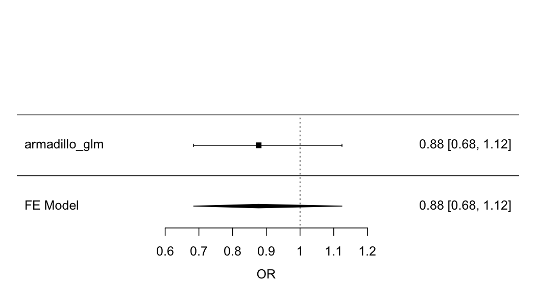
plot of chunk meta-analysis
Creating figures
You can directly create figures with the DataSHIELD methods. For example:
# create histogram
ds.histogram(x = "core_nonrep$coh_country", datasources = conns)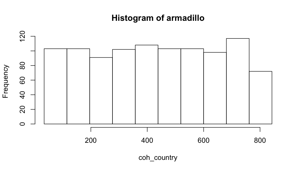
plot of chunk create-a-histogram
#> $breaks
#>  [1]  35.31138 116.38319 197.45500 278.52680 359.59861 440.67042 521.74222 602.81403 683.88584 764.95764
#> [11] 846.02945
#>
#> $counts
#>  [1] 106 101  92 103 106 104 105 101 113  69
#>
#> $density
#>  [1] 0.0013074829 0.0012458092 0.0011347965 0.0012704787 0.0013074829 0.0012828134 0.0012951481
#>  [8] 0.0012458092 0.0013938261 0.0008510974
#>
#> $mids
#>  [1]  75.84729 156.91909 237.99090 319.06271 400.13451 481.20632 562.27813 643.34993 724.42174 805.49355
#>
#> $xname
#> [1] "xvect"
#>
#> $equidist
#> [1] TRUE
#>
#> attr(,"class")
#> [1] "histogram"
# create a heatmap
ds.heatmapPlot(x = "analysis_df$pets_.1", y = "analysis_df$dogs_.1", datasources = conns)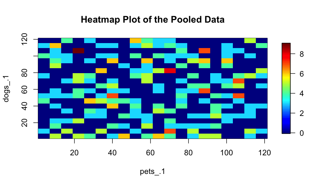
plot of chunk create-a-heatmap
# logout
datashield.logout(conns)